Backblaze hard disk drive failure data: Update to Q2 2016
Ross Lazarus, September 2016
This is a Kaplan Meier analysis of the BackBlaze hard drive reliability data, using all available data to end second quarter of 2016 from https://www.backblaze.com/b2/hard-drive-test-data.html .
Previous posts are at http://bioinformare.blogspot.com.au/2016/05/survival-analysis-of-hard-disk-drive.html and http://bioinformare.blogspot.com.au/2016/02/survival-analysis-of-hard-disk-drive.html .
I reran my scripts and got the plots shown below. It's taking a while to read all the data as there are now a very large number of drives spinning. A total of 41740623 rows were processed in about 35 minutes on my home desktop by the python script in the github repository.
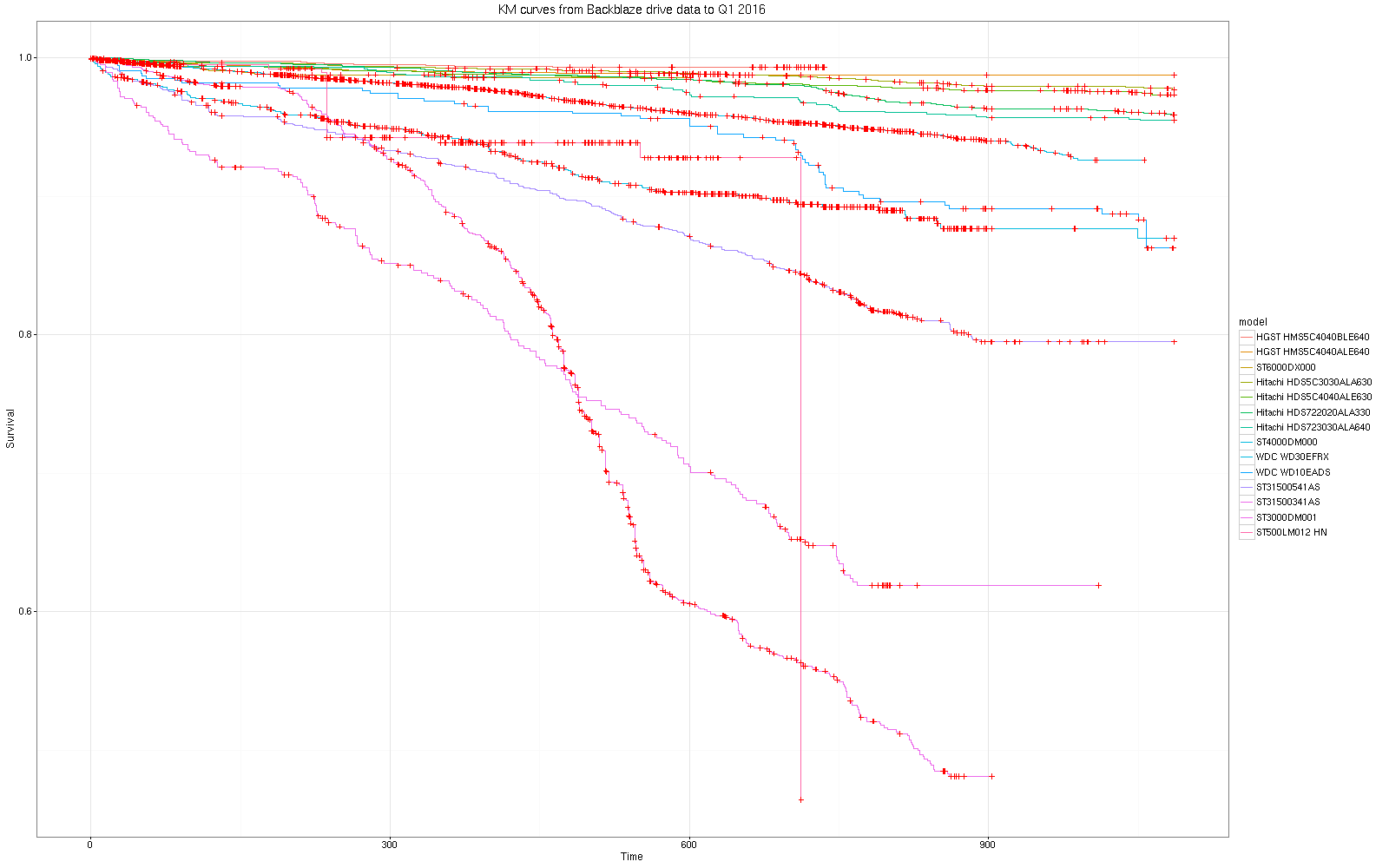
Updated curves:
and
By Manufacturer:
 |
| Add caption |
Once again for me, little change is seen in the KM curves and statistics with a lot more drives and a lot more observaton time, suggesting that this statistical approach is reliable and robust, although in general we expect that more data provides better resolution.
In terms of the KM statistical tests, additional data confirms the earlier inference that there are significant differences between the manufacturer and model risk profiles over time.
Call:
survdiff(formula = sm ~ model, data = dm, rho = 0)
N Observed Expected (O-E)^2/E (O-E)^2/V
model=HGST HMS5C4040ALE640 7168 85 505.51 349.800 406.826
model=HGST HMS5C4040BLE640 8505 29 269.99 215.103 231.736
model=Hitachi HDS5C3030ALA630 4664 117 466.48 261.826 302.989
model=Hitachi HDS5C4040ALE630 2719 71 268.60 145.365 157.458
model=Hitachi HDS722020ALA330 4774 215 472.27 140.149 161.908
model=Hitachi HDS723030ALA640 1048 55 103.54 22.753 23.459
model=ST3000DM001 4707 1705 246.40 8634.322 9272.385
model=ST31500341AS 787 216 35.74 909.141 917.789
model=ST31500541AS 2188 392 157.42 349.574 363.940
model=ST4000DM000 36089 1123 1500.66 95.042 151.313
model=ST500LM012 HN 801 26 22.42 0.573 0.577
model=ST6000DX000 1915 31 77.14 27.601 28.497
model=ST8000DM002 2754 3 3.74 0.146 0.149
model=WDC WD10EADS 550 60 46.72 3.773 3.818
model=WDC WD30EFRX 1289 136 87.38 27.053 27.637
Chisq= 11353 on 14 degrees of freedom, p= 0
Call:
survdiff(formula = s ~ manufact, data = ds, rho = 0)
N Observed Expected (O-E)^2/E (O-E)^2/V
manufact=HGST 15840 120 821.8 599.348 744.193
manufact=Hitachi 13246 462 1433.5 658.440 1046.810
manufact=HN 801 26 23.6 0.242 0.243
manufact=ST 49900 3792 2255.7 1046.249 2067.849
manufact=TOSHIBA 279 12 13.6 0.181 0.182
manufact=WDC 3920 385 248.7 74.701 78.874
Chisq= 2493 on 5 degrees of freedom, p= 0


I am glad to find this article useful for me because it is very informative. I found this in your post. Thanks for sharing
ReplyDeletewordpress
ufa88kh.blogspot
youtube
SA GAMING
Very Informative blogs. If you want to promote your business… with just one click we can give sales leads
ReplyDeleteNO DLT, NO APPROVAL REQUIRED
Wholesale Pricing
24/7 Support
Pay as you GO
No Setup & Monthly Fees
bulk sms in bangalore | bulk sms explicit Bangalore | promotional sms provider | bulk sms reseller mysuru | SMS API | bulk sms gateway | sms implicit
I love your posts and everything looks wonderful. I love your idea thanks for sharing.
ReplyDeletewordpress
blogspot
youtube
មាន់ជល់
This comment has been removed by the author.
ReplyDeleteThank you for sharing such a valuable and insightful article!
ReplyDeleteYour perspectives on technology and digital transformation are incredibly helpful for businesses aiming to scale and innovate with confidence.
If you’re interested in exploring more expert-led content on technology, AI, software solutions, automation, and digital strategy, we invite you to visit our website:
👉 Nexxora Inc
At Nexxora, we publish in-depth blogs and industry insights covering:
Cloud Solutions & IT Consulting
Advanced Digital Transformation
Custom Software Development
Business Process Automation
Data-Driven Growth Strategies
We also provide end-to-end digital and IT services. Whether you need consulting, application development, branding, or automation solutions, our team is here to help.
Feel free to connect with us anytime — we’d be delighted to collaborate and support your business growth.