Survival analysis of hard disk drive failure data: Update to Q1 2016
Ross Lazarus, May 2016
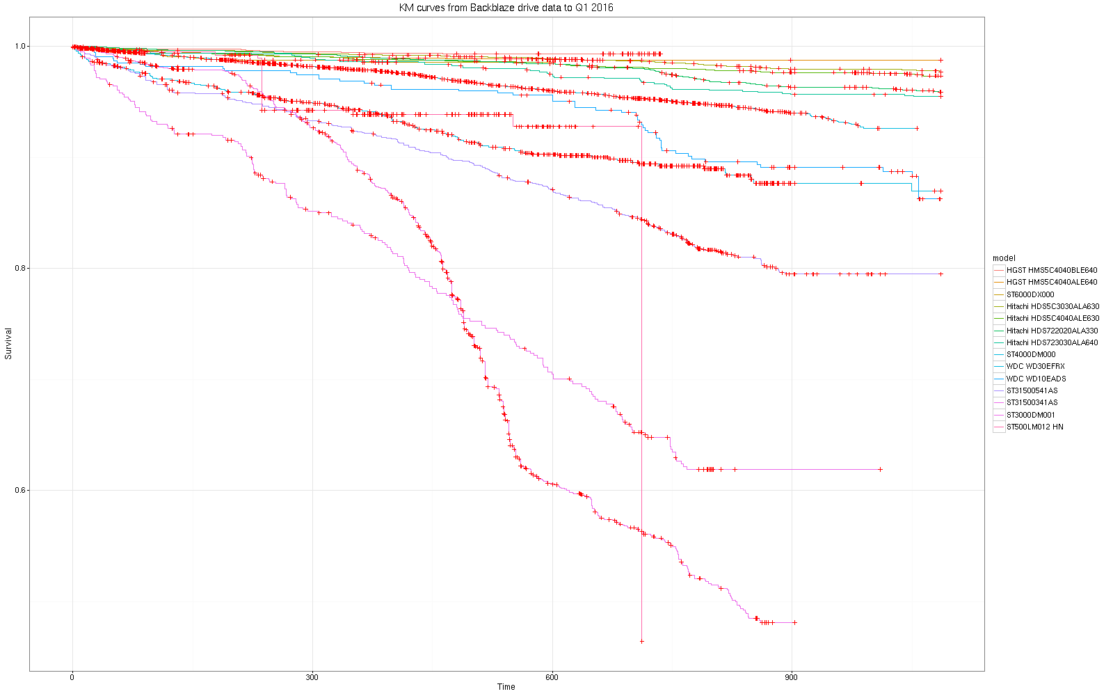
This is an update to http://bioinformare.blogspot.com.au/2016/02/survival-analysis-of-hard-disk-drive.html now that additional data for Q1 2016 has been released from https://www.backblaze.com/b2/hard-drive-test-data.html.I reran my scripts and got the plots shown below. Whole process only takes a few minutes.
For me, the interesting thing is that so little really changes in the KM curves and statistics with 10% more data, suggesting that this statistical approach is reliable and robust, although in general we expect that more data provides better resolution.
The WD30-EFRX and WD10-EADS and drives are reordered in terms of failure risk with more data down near the middle of the pack, but the updated models KM curves otherwise suggest the same pattern of risk of failure over time. Hitachi and HGST have reversed their positions at the top of the manufacturer survival curves as a result of the additional data, but the other manufacturers remain largely unchanged.
In terms of the KM statistical tests, additional data confirms the earlier inference that there are significant differences between the manufacturer and model risk profiles over time.
Call:
survdiff(formula = sm ~ model, data = dm, rho = 0)
N Observed Expected (O-E)^2/E (O-E)^2/V
model=HGST HMS5C4040ALE640 7168 83 473.2 321.78 376.18
model=HGST HMS5C4040BLE640 3115 21 231.4 191.29 205.14
model=Hitachi HDS5C3030ALA630 4664 106 458.0 270.51 313.62
model=Hitachi HDS5C4040ALE630 2719 70 263.4 141.98 153.89
model=Hitachi HDS722020ALA330 4774 195 466.4 157.94 183.39
model=Hitachi HDS723030ALA640 1048 47 101.7 29.42 30.35
model=ST3000DM001 4707 1705 258.4 8100.00 8753.25
model=ST31500341AS 787 216 37.8 839.35 848.18
model=ST31500541AS 2188 392 166.0 307.66 321.95
model=ST4000DM000 35858 895 1302.4 127.45 195.39
model=ST500LM012 HN 656 24 17.2 2.70 2.71
model=ST6000DX000 1909 26 57.4 17.19 17.76
model=WDC WD10EADS 550 59 47.5 2.78 2.81
model=WDC WD30EFRX 1280 124 82.2 21.26 21.72
Chisq= 10647 on 13 degrees of freedom, p= 0
Call:
survdiff(formula = s ~ manufact, data = ds, rho = 0)
N Observed Expected (O-E)^2/E (O-E)^2/V
manufact=HGST 10449 110 740.5 536.857 668.750
manufact=Hitachi 13246 422 1380.6 665.600 1060.350
manufact=HN 656 24 18.2 1.885 1.896
manufact=ST 46909 3507 2032.7 1069.209 2056.135
manufact=TOSHIBA 255 10 11.3 0.154 0.155
manufact=WDC 3838 342 231.7 52.560 55.539
Chisq= 2420 on 5 degrees of freedom, p= 0
Here are the updated curves:


This comment has been removed by the author.
ReplyDeleteYour approach is only reliable and robust if you have actual experience in the HDD segment and understand how flawed the data set from Backblaze is, I can list the reasons if you are interested. Also, comparing a sample size of 20,000 or 30,000 drives to a sample size of either 250(Toshiba) or 2-3K(WD) is terrible practice for "reliable" statistical results.(I really wanted to use some harsher words here, but I will not).
ReplyDeleteThanks for your thoughts. Even better would be if you could share some of your extensive experience and skill by showing us how to do it better? Constructive, informed criticism is always welcome.
DeleteYes, there's less information with fewer drives but that doesn't alter the utility of this old method which is all I'm trying to demonstrate here. Sample size for each curve is obvious - hint, each censored observation is a "+" - and the KM statistics take it into account as you'll see if you take the time to read up on the method.
Why do some of the curves level out to flat at the end, even though there seem to be data points indicating failures in the flat portions?
ReplyDeleteAre you confusing the + signs (which indicate when a unit was censored - ie removed from the study when still functioning) with failure times when the curve must fall because the y axis is fraction of drives known not to have failed ('survival') which by definition has to decrease when a failure occurs. Censoring has no effect on our estimate of survival since it was lost to observation so we don't know when or even if a censored drive failed. You may need to read up more on the problems of right censored data and the Kaplan-Meier curve and statistic.
DeleteYou are correct that I thought the + signs were failures, not removals. Thanks for the explanation.
DeleteDrive failure rates are much, much lower than the density of censoring. It's one of the more uncertain aspects of this data - that drives might have been pulled from pods and thus censored when in fact they were starting to show signs (eg smartdrive stats?) of impending doom....but that's a universal problem with this kind of right censored data and the KM method is about as good as it gets in terms of robust statistical approaches with no distributional assumptions - which is why I thought it made sense here compared to the tables and bar charts Backblaze and others have published - which I find hard to interpret - the KM curves make things fairly clear to me....
DeleteHello, sorry for my ignorance, what is that V in (O-E)^2/V? Is the expected values calculated only from the backblaze dataset? What can we understand from the high normalized (O-E)^2/E values? That (for example) HGST drives have unpredictable failure rates? What's the meaning of Chisquared (on n degrees of freedom)? Is a censored drive a drive removed from the analysis or even a drive pulled out of a server and then put back inside?
ReplyDeleteThanks for your insight, in this article and your previous one, I've never read anything that takes this approach to hdd failure rates, I agree this representation is much more interesting or probably more correct (eg aligning each device observation history in t=0, instead of looking at time frames, which, after seeing your article, IMHO really does not make any sense)
V represents the variance of (obs - expected) so that's the log rank test for curve differences - numerically it varies slightly from the chisquared test and is also a valid test. You will probably want to read up on the method. Thishttps://stat.ethz.ch/education/semesters/ss2011/seminar/contents/presentation_2.pdf has a pretty good explanation but sadly it's still statistics
ReplyDelete:)
Thanks for this in-depth analysis, detailed description of your arguments and your update (will there be more?). I totally agree with you that this improves the view on the reliability of the hard disks. Also tribute to Backblaze because of publishing their data and conclusions.
ReplyDeleteOne thing is however is not clear to me. About the HDDs which have been replaced by Backblaze because the smart statistics showed values above Backblazes thresholds (so they would probably fail soon): are they considered as 'failure' or as 'censored' (you said: "I don't trust the smartdrive stats"). I hope they are handled as 'failure' because it's like a patient who is sent home alive with the message that he will die soon. Whether these disks are actually broken or not doesn't matter anymore, for Backblaze their life is over.
Jack
PS Sorry for my English. it's not my native language.
Hi - thanks for caring - I reran the scripts with the new data - http://bioinformare.blogspot.com.au/2016/09/backblaze-hard-disk-drive-failure-data.html
DeleteInteresting - thanks for provoking me into updating it.
Those guys are backblaze are smart but they're not using the data right I think - or else they are being cagey - their analysis https://www.backblaze.com/blog/hard-drive-failure-rates-q2-2016/ seems to minimise the rather obvious low failure rate over all the available data for those 8tb seagates - they only show a single quarter at a time? I can't imagine why since there's so much more information there.
Have you 1) published your scripts? 2) looked at 2017 data?
ReplyDeleteSource was published at https://github.com/fubar2/backblazeKM
ReplyDeletePull requests welcomed.
Yes, I have run the most up to date data. Very little change gratifyingly enough.
ta. Excellent. From what BB say, they consider a disk as failed if one of 5(?) SMART thresholds are exceeded. Doesn't this mean that we can be confident that a removed disk is one that has failed or will fail and this is what we want to know about had disk reliability?
DeleteDunno.
ReplyDeleteI started parsing those smartdrive stats but there was mucho missing data so I chose to go with the simplest definition of survival - but yes, there must be confounding - OTOH they retire drive pods for other reasons so this all is rather inexact. Never mind the quality, feel the width comes to mind.
Good
ReplyDelete...................
goldenslot
golden slot